Here is what we are going to cover:

• The need for liquidity
• A basic foundation to understand how liquidity is seeded when a pool is launched
• Incentivizing for liquidity
• Understanding concentrated liquidity and its implications on impermanent loss.

Curve finance is referenced a lot in explaining the liquidity incentives and leveraged liquidity. The information is super basic and foundational to understanding the complex mechanics behind the protocols and it is the first article in a series of articles dedicated to Curve Finance.

If this simple reading layout doesn’t excite you, you could scroll down to consume the same content as if it were a magazine.

⚠ Disclaimer: All information presented here is my perspective and should be considered educational content. I won’t be responsible for any kind of financial profits or losses derived from your decisions. Financial and investment advice

May it be traditional finance or Defi, any tradable asset needs liquidity to gain adoption. All Defi protocols more or less have their native token as a mode of value accrual just like shares of the company in the traditional finance ecosystem. Unlike shares in traditional finance, tokens prove to have more use cases.

Why Liquidity?

For any protocol to be scalable the native token of that particular protocol must be liquid enough to tank the price fluctuation.

If the liquidity depth is less, the price shifts due to the trades will be high which means higher volatility. Nobody wants to own an extremely uncertain asset as it can be easily manipulated even though lesser volume trades.

When a trade occurs of 1000 ABC for XYZ in a pair ABC / XYZ with TVL 2,000,000 and pricing at 1, the price after the trade will be 0.998. The price impact of almost 0.2%.

When a trade occurs of 1000 ABC for XYZ in a pair ABC / XYZ with TVL 20,000 and pricing at 1, the price after the trade will be 0.826. The price impact of almost 17.35%.

Controlling the liquidity is more crucial for the protocol than the traders or the holders. In simple terms, liquidity can make or break a protocol.

Protocol’s Perspective: Seeding Liquidity

Buying the Liquidity

There are ways to acquire liquidity and manage it. The easiest way to provide liquidity is to buy the tokens and provide liquidity in a liquidity pool.

Buying an equivalent worth of another token to pair with the protocol’s native token for the purpose of establishing liquidity is one of the most ineffective ways to supply liquidity for the protocol itself. In the scenario discussed, the protocol is betting on scalability as well as the appreciation of the other token to make sure they are not losing on the initial investment.

As in the business world, you always use others’ money in order to generate value, Defi withholds the same concept.

Inflation as Rewards

The second way to ensure liquidity is to inflate your native token and distribute that inflation to incentivize the people who choose to provide liquidity for your native token.

This is the most used model to fund or own liquidity in the Defi ecosystem. This model includes inducing incentives for others to provide liquidity for you. This can be executed by directing your native token’s inflation to the people providing liquidity.

Non-volatile Rewards

You can even establish a strategic position where liquidity providers get favorable incentives that are less riskier for the liquidity providers to hold. This approach is much more favorable as the native token of the protocol won’t be stable enough to be distributed as an incentive, it would just increase the selling pressure on the native token just like the other farm tokens.

Curve finance is a platform that aligns with the above approach. It distributes $CRV along with other incentives from trading fees, the distribution of $CRV is a bit complex to understand and it will be covered in a further section in complete detail.

Managing Liquidity

Addressing the Sell Pressure on Farm Tokens

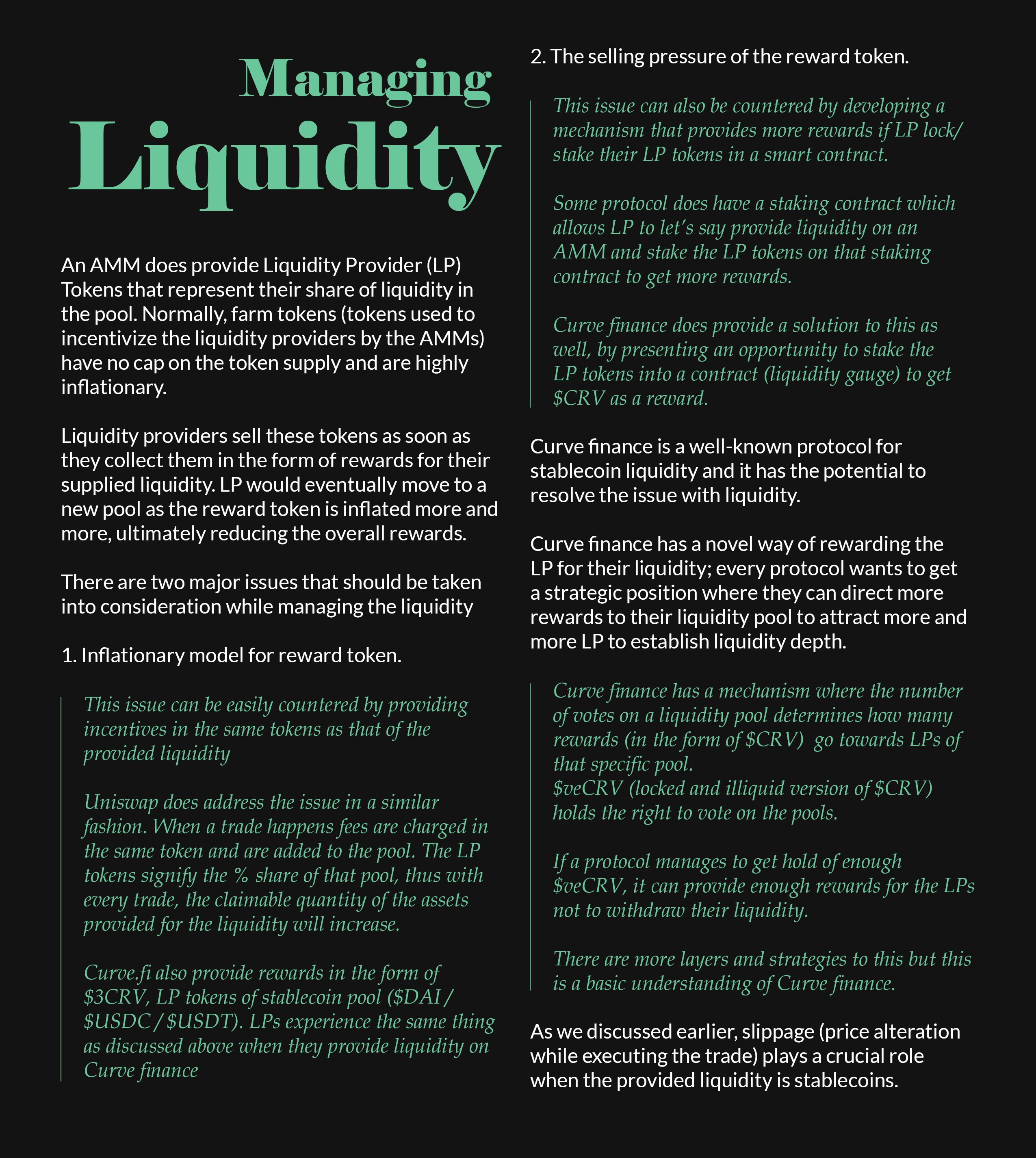
An AMM does provide Liquidity Provider (LP) Tokens that represent their share of liquidity in the pool. Normally, farm tokens (tokens used to incentivize the liquidity providers by the AMMs) have no cap on the token supply and are highly inflationary.

Liquidity providers sell these tokens as soon as they collect them in the form of rewards for their supplied liquidity. LP would eventually move to a new pool as the reward token is inflated more and more, ultimately reducing the overall rewards.

There are two major issues that should be taken into consideration while managing the liquidity

• Inflationary model for reward token.

This issue can be easily countered by providing incentives in the same tokens as that of the provided liquidity

Uniswap does address the issue in a similar fashion. When a trade happens fees are charged in the same token and are added to the pool. The LP tokens signify the % share of that pool, thus with every trade, the claimable quantity of the assets provided for the liquidity will increase.

Curve.fi also provide rewards in the form of $3CRV, LP tokens of stablecoin pool ($DAI / $USDC / $USDT). LPs experience the same thing as discussed above when they provide liquidity on Curve finance.

• The selling pressure of the reward token.

This issue can also be countered by developing a mechanism that provides more rewards if LP lock/stake their LP tokens in a smart contract.

Some protocol does have a staking contract which allows LP to let’s say provide liquidity on an AMM and stake the LP tokens on that staking contract to get more rewards.

Curve finance does provide a solution to this as well, by presenting an opportunity to stake the LP tokens into a contract (liquidity gauge) to get $CRV as a reward.

Approach by Curve Finance

Curve finance is a well-known protocol for stablecoin liquidity and it has the potential to resolve the issue with liquidity.

Curve finance has a novel way of rewarding the LP for their liquidity; every protocol wants to get a strategic position where they can direct more rewards to their liquidity pool to attract more and more LP to establish liquidity depth.

Curve finance has a mechanism where the number of votes on a liquidity pool determines how many rewards (in the form of $CRV) go towards LPs of that specific pool. $veCRV (locked and illiquid version of $CRV) holds the right to vote on the pools.

If a protocol manages to get hold of enough $veCRV, it can provide enough rewards for the LPs not to withdraw their liquidity.

There are more layers and strategies to this but this is a basic understanding of Curve finance.

As we discussed earlier, slippage (price alteration while executing the trade) plays a crucial role when the provided liquidity is stablecoins.

Leveraged Liquidity aka Concentrated Liquidity

Stablecoins are meant to be pegged to $1 UDS and are supposed to be non-volatile.

Curve finance uses these traits as leverage to create the concept of concentrated liquidity which in turn provides low slippage to traders and meanwhile, the stablecoins remain non-volatile.

Understanding the Segmentation of a Liquidity Pool

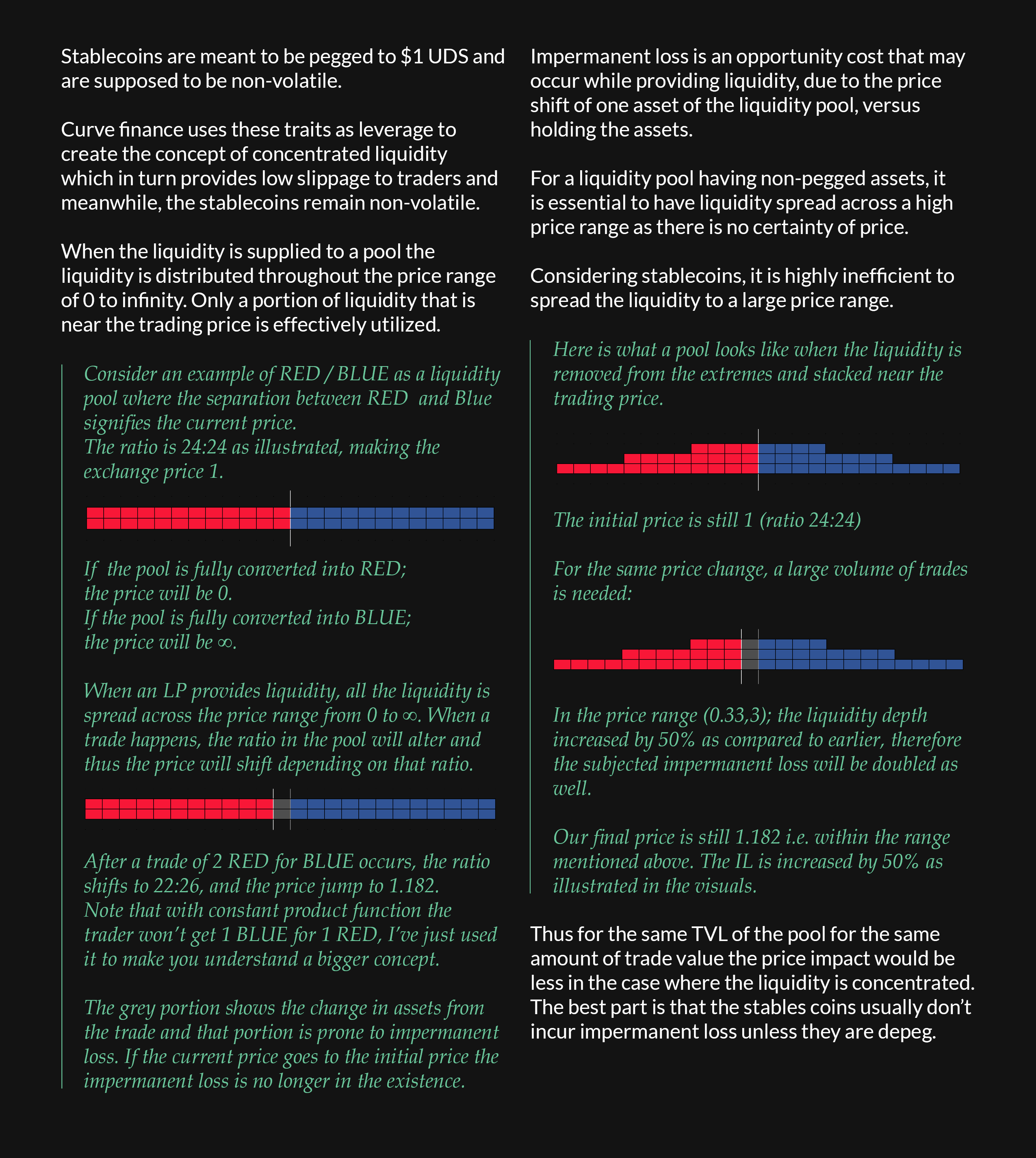
When the liquidity is supplied to a pool the liquidity is distributed throughout the price range of 0 to infinity. Only a portion of liquidity that is near the trading price is effectively utilized.

Consider an example of RED / BLUE as a liquidity pool where the separation between RED and Blue signifies the current price. The ratio is 24:24 as illustrated, making the exchange price 1.

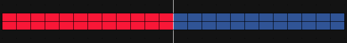
If the pool is fully converted into RED; the price will be 0.

If the pool is fully converted into BLUE; the price will be ∞.

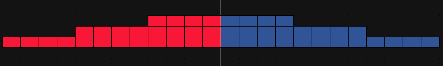
When an LP provides liquidity, all the liquidity is spread across the price range from 0 to ∞. When a trade happens, the ratio in the pool will alter and thus the price will shift depending on that ratio.

After a trade of 2 RED for BLUE occurs, the ratio shifts to 22:26, and the price jump to 1.182. Note that with constant product function the trader won’t get 1 BLUE for 1 RED, I’ve just used it to make you understand a bigger concept.

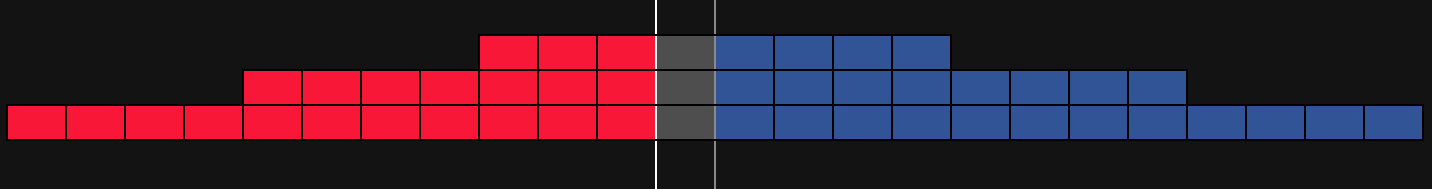
The grey portion shows the change in assets from the trade and that portion is prone to impermanent loss. If the current price goes to the initial price the impermanent loss is no longer in the existence.

Impermanent loss is an opportunity cost that may occur while providing liquidity, due to the price shift of one asset of the liquidity pool, versus holding the assets.

For a liquidity pool having non-pegged assets, it is essential to have liquidity spread across a high price range as there is no certainty of price.

Considering stablecoins, it is highly inefficient to spread the liquidity to a large price range.

Redistribution of the Assets in the Liquidity Pool

Here is what a pool looks like when the liquidity is removed from the extremes and stacked near the trading price.

The initial price is still 1 (ratio 24:24) For the same price change, a large volume of trades is needed:

In the price range (0.33,3); the liquidity depth increased by 50% as compared to earlier, therefore the subjected impermanent loss will be doubled as well.

Our final price is still 1.182 i.e. within the range mentioned above. The IL is increased by 50% as illustrated in the visuals.

Thus for the same TVL of the pool for the same amount of trade value the price impact would be less in the case where the liquidity is concentrated. The best part is that the stables coins usually don’t incur impermanent loss unless they are depegged.

Thank you for being here.

You can provide the same value by sharing this article with your circle.

You could even contribute/support these articles by owning one ✌.

Thank you for being here.

You can provide the same value by sharing this article with your circle.

You could even contribute/support these articles by owning one ✌.